
Bienvenue dans ce chapitre sur le calcul de prévision des ventes !
Voici les 4 méthodes que je vais aborder dans ce cours de Gestion opérationnelle pour le BTS MCO :
- Méthode N°1 : La méthode des moindres carrés
- Méthode N°2 : La méthode des points extrêmes
- Méthode N°3 : La méthode de Mayer ou Méthode de la double moyenne
- Méthode N°4 : La saisonnalité des ventes
- Le coefficient de corrélation et la prévision des ventes
- Conclusion
Quelle que soit la méthode de prévision, le principe général est le même.
À l’aide d’une droite d’équation de la forme « y = ax+b », il s’agit de trouver les chiffres d’affaires futurs.
Tout au long de cet article je vais prendre l’exemple suivant :
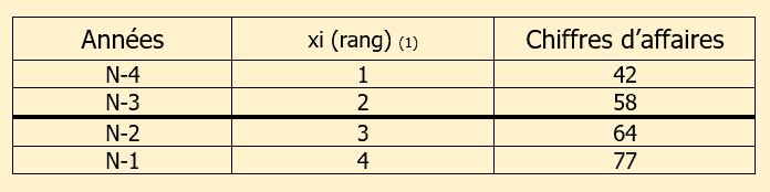
On donne le tableau suivant concernant les informations financières d’un magasin de restauration rapide dans la banlieue parisienne. Vous devez étudier la prévision de ces données pour l’année N+1.
| Années | Chiffres d'affaires |
|---|---|
| N-4 | 42 |
| N-3 | 58 |
| N-2 | 64 |
| N-1 | 77 |
Lorsque vous rédigez un exercice, vous devez bien faire attention à l’ordre chronologique.
Sommaire
Méthode N°1 : La méthode des moindres carrés
Dans cette méthode de prévision des ventes d’ajustement linéaire, on pose les éléments suivants :
- la période considérée soit « xi »
- le chiffre d’affaires correspond à « yi »
- le nombre de lignes du tableau des éléments passés correspond à « n »
Avec les éléments précédents, vous devez calculer deux moyennes : la moyenne des périodes et la moyenne des chiffres d’affaires.
Le terme moyenne est identifié à l’aide d’une petite barre sur la lettre comme dans les formules suivantes.
Pour cela, vous devez appliquer les formules qui suivent :
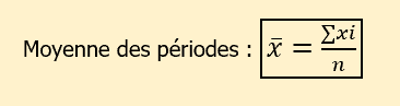
La formule de la moyenne des périodes que l’on appelle « moyenne de x » :
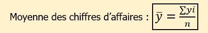
La formule de la moyenne des chiffres d’affaires que l’on appelle « moyenne de y » :
Comment lire les formules ?
La lecture de la formule des moyennes des périodes est la suivante :
moyenne de « x » égal somme des « xi » divisée par « n »
La lecture de la formule des moyennes des chiffres ‘affaires est la suivante :
moyenne de « y » égal somme des « yi » divisée par « n »
Dans un premier temps, vous ne pouvez pas appliquer de formules pour trouver ces deux moyennes. Vous devez passer par l’élaboration d’un tableau préparatoire.
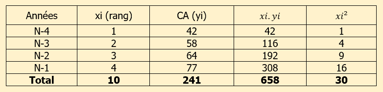
Voici un exemple de tableau préparatoire qui va vous aider à trouver les éléments utiles :
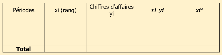
La ligne la plus importante du tableau est la ligne « Total ».
Le »Rang » correspond à un chiffre que l’on attribue à une période afin de pouvoir s’en servir pour appliquer une formule.
Il faut toujours commencer par le chiffre « 1 » pour la période la plus lointaine et incrémenter (augmenter) de « 1 » pour chaque nouvelle période.
Le total de la colonne « xi » est utile pour calculer la moyenne des périodes. Le total de la colonne « yi » est utile pour le calcul des moyennes des chiffres d’affaires.
Je vais appliquer les formules avec les éléments chiffrés de notre exemple de départ.
Dans notre exemple « n » = 4 car il y a quatre lignes dans le tableau de l’énoncé.
La formule de la moyenne de x est la suivante :
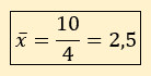
Et la moyenne de y est :
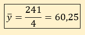
Ce même tableau sert également à calculer d’autres formules.
Comment calculer les paramètres « a » et « b » de l’équation ?
Pour déterminer l’équation de la droite de la forme « y=ax+b », il est nécessaire de trouver dans un premier temps les paramètres de l’équation, c’est-à-dire l’élément « a » et l’élément « b ».
C’est là qu’interviennent les totaux des colonnes « xi.yi » et « xi au carré ».
« xi.yi » signifie xi multiplié par yi. Ce calcul est fait pour chaque ligne du tableau.
« xi » au carré signifie que pour chaque ligne de « xi » du tableau la valeur est mise au carré.
Pour trouver les paramètres « a » et « b » il faut appliquer les formules suivantes :
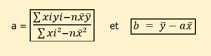
Dans la formule du paramètre « a », nous avons les éléments suivants :
- la somme du produit « xi.yi »
- le nombre de lignes du tableau « n »
- la somme de la colonne « xi au carré »
- les moyennes de x et de y
Dans la formule du paramètre « b », nous avons les moyennes de x et de y d’une part, et d’autre part le paramètre « a ».
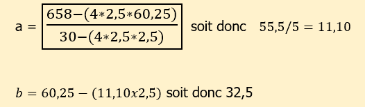
Voici donc ce que cela donne dans notre exemple :
Maintenant nous pouvons appliquer les formules des paramètres « a » et « b » :
Comment interpréter les paramètres « a » et « b » ?
Pour interpréter les valeurs trouvées, il faut remplacer « a » et « b » dans l’équation « y = ax + b » par ces mêmes valeurs :
y = 11,10x + 32,5
On peut donc écrire que cette équation permet de trouver n’importe quels chiffres d’affaires futurs (c’est à dire prévisionnels).
Comment réaliser la prévision des ventes ?
Une fois l’équation déterminée, on doit remplacer « x » par le rang de la période recherchée. Dans notre exemple le rang de la période recherchée est 6.
Pourquoi « 6 » ? Dans notre tableau initial, le dernier rang est 4 correspondant à la l’année « N-1 ».
Donc l’année N correspond au rang 5 et l’année N+1 correspond bien au rang 6.
D’où l’équation suivante :
y = (11,10 x 6) + 32,5 = 99,10
Nous pouvons donc écrire que le chiffre d’affaires prévisionnel pour l’année N+1 est de 99,10 K€.
Méthode N°2 : Prévision des ventes par la méthode des points extrêmes
Quel est le principe de la méthode ?
Cette méthode d’ajustement linéaire de prévision des ventes consiste à prendre en considération la période la plus ancienne et la période la plus récente, à poser un système d’équations, à trouver les paramètres de ce système, et enfin à réaliser la prévision.
Rappel du tableau initial de l’exercice :
| Années | Chiffres d'affaires |
|---|---|
| N-4 | 42 |
| N-3 | 58 |
| N-2 | 64 |
| N-1 | 77 |
Comment poser un système d’équations ?
Voici la méthode à suivre pour poser correctement le système d’équations :
- identifier les deux lignes concernées : la plus ancienne et la plus récente
- la colonne Chiffres d’affaires représente les « yi »
- la colonne « Rang » représente les « xi »
- les équations recherchées sont de la forme : y = ax + b
- Remplacez « x » et « y » par « xi » et « yi » pour les deux lignes concernées
Dans notre exemple nous avons le système d’équations suivant :
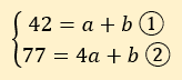
Pour résoudre ce système d’équations il existe plusieurs méthodes. Nous utiliserons la méthode par soustraction. Nous allons retrancher membre à membre la première équation à la seconde équation.
77 = 4a + b
42 = a + b
_________
35 = 3a
En effet : 77 – 42 = 35 et 4a – a = 3a et « b » – « b » = 0b
35 = 3a devient :
a = 35/3
a = 11,66
Nous venons de trouver la valeur de « a ». Pour trouver la valeur de « b », il faut remplacer « a » dans l’une des deux équations de départ.
Prenons par exemple la première équation : 42 = a + b
On a donc :
42 = 11,66 + b
b = 42 – 11,66
b = 31,66
Maintenant que nous avons les deux paramètres de l’équation y = ax + b, nous pouvons écrire l’équation qui permet de trouver n’importe quels chiffres d’affaires prévisionnels :
y = 11,66x + 31,66
Calcul de la prévision des ventes
Nous remplaçons « x » par le rang de la période recherchée, soit dans notre exemple le rang 6 qui correspond à l’année N+1 :
y = (11,66 x 6) + 31,66
y = 69,96 + 31,66
y = 101,62 K€
On peut donc en conclure que le chiffre d’affaires prévisionnel N+1 s’élève à 101,62 K€.
Voici une vidéo sur la méthode des points extrêmes.
Méthode N°3 : La méthode de Mayer ou Méthode de la double moyenne
Quel est le principe de la méthode ?
Cette méthode de prévision des ventes d’ajustement linéaire consiste à diviser la série statistique en deux sous catégories en parts égales (si possible).
Pour chacune d’elle, on détermine les moyennes et une équation de la forme y = ax+b.
Enfin on résoudra un système d’équations, on trouvera les paramètres « a » et « b » puis nous réaliserons la prévision N+1.
Tout d’abord, je partage la série statistique en deux sous catégories :
Calculs des moyennes et détermination de l’équation
Première sous-catégorie :
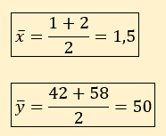
Pour écrire l’équation de la forme y = ax + b, je remplace « x » et « y » par les moyennes.
D’où l’équation qui s’écrit : 50 = 1,5a + b
Seconde sous-catégorie :
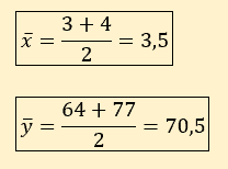
D’où l’équation qui s’écrit : 70,5 = 3,5a + b
Résolution du système d’équation
le système d’équation est le suivant :
50 = 1,5a + b
70,5 = 3,5a + b
Pour résoudre ce système d’équations il existe plusieurs méthodes. Nous utiliserons la méthode par soustraction. Nous allons retrancher membre à membre la première équation à la seconde équation.
70,5 = 3,5a + b
50 = 1,5a + b
____________
20,5 = 2a
En effet, 70,5 – 50 = 20,5 ; 3,5a – 1,5a = 2a et b – b = 0b
Nous avons donc :
20,5 = 2a
a = 20,5/2
a = 10,25
Pour trouver la valeur de « b », nous remplaçons « a » dans l’une des deux équations de départ.
je vais prendre la première équation :
50 = 1,5a + b
50 = (1,5 x 10,25) + b
50 = 15,375 + b
b = 50 – 15,375
b = 34,625
Nous pouvons donc écrire :
L’équation de la droite d’ajustement qui permet de trouver n’importe quels chiffres d’affaires prévisionnels s’écrit :
y = 10,25x + 34,625
Calcul de la prévision des ventes
Nous remplaçons « x » par le rang de la période recherchée, soit dans notre exemple le rang 6 qui correspond à l’année N+1 :
y = (10,25 x 6) + 34,625
y = 61,5 + 34,625
y = 96,125
On peut donc en conclure que le chiffre d’affaires prévisionnel N+1 s’élève à 96,125 K€.
La saisonnalité des ventes
Le principe de la saisonnalité des ventes
Le principe consiste à déterminer les chiffres d’affaires futurs en tenant compte des variations saisonnières qui sont elles-mêmes fonction de l’activité de l’entreprise.
Il existe de nombreuses méthodes pour calculer les coefficients saisonniers (On partira du principe que les chiffres d’affaires donnés sont trimestriels et que l’on possède le chiffre d’affaires prévisionnel).
Comment calculer le coefficient de saisonnier ?
Prévision des ventes : La méthode des pourcentages
Voici les différentes étapes de calculs que vous devez insérer dans des colonnes du tableau final :
- calcul du chiffre d’affaires total
- calcul de la proportion du chiffre d’affaires pour chaque période
- calcul du chiffre d’affaires prévisionnel pour chaque période
En reprenant notre exemple et en tenant compte des précisions indiquées plus haut, nous avons les calculs suivants :
Total des ventes de l’année N : 241 K€
Calcul de la proportion des ventes pour chaque trimestre :
Trimestre 1 : 42 ÷ 241 = 0,17 soit 17%
Trimestre 2 : 58 ÷ 241 = 0,24 soit 24%
Trimestre 3 : 64 ÷ 241 = 0,26 soit 26%
Trimestre 4 : 77 ÷ 241 = 0,33 soit 33%
La somme des coefficients donne 1.
Calcul de la prévision :
Pour réaliser la prévision vous devez multiplier le chiffre d’affaires prévisionnel annuel par le coefficient saisonnier du trimestre considéré.
La prévision s’effectue par période et dans notre exemple il s’agit du trimestre.
Voici donc les calculs :
Dans l’énoncé on donne également l’information suivante : le chiffre d’affaires N+1 est de 300 K€.
Trimestre 1 : 300 x 0,17 = 51
Trimestre 2 : 300 x 0,24 = 72
Trimestre 3 : 300 x 0,26 = 78
Trimestre 4 : 300 x 0,33 = 99
La somme des prévisions est égale au chiffre d’affaires prévisionnel N +1 soit 300 K€.
Interprétation des résultats
Par exemple pour le second trimestre, l’interprétation est : Le chiffre d’affaires prévisionnel du deuxième trimestre N + 1 est de 72 K€.
Prévision des ventes : La méthode des moyennes
Principe de la méthode des moyennes
Cette méthode consiste à calculer la moyenne des périodes, puis à calculer le coefficient saisonnier et finalement à déterminer la prévision des ventes.
Voici un exemple de calcul selon la méthode des moyennes.
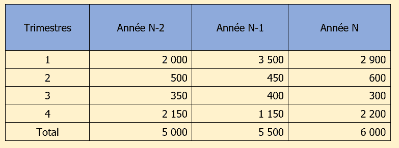
L’énoncé précise que le chiffre d’affaires annuel prévisionnel est de 6 500 K€ et donne le tableau suivant :
Comment calculer le coefficient saisonnier ?
Voici les différentes étapes de calculs que vous devez insérer dans des colonnes du tableau final :
- réaliser la moyenne des chiffres d’affaires par période (en ligne)
- calculer la moyenne des moyennes
- calculer le coefficient saisonnier en rapportant chaque moyenne sur la moyenne des moyennes
Calcul de la moyenne des chiffres d’affaires par période en ligne :
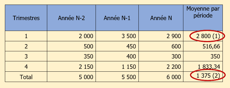
(1) : (2 000 + 3 500 + 2 900) / 3 = 2 800 et ainsi de suite pour chaque période (ligne)
(2) : (2 800 + 516,66 + 350 + 1 833,34) / 4 = 1 375
Le coefficient se calcule en divisant la moyenne d’un trimestre par la moyenne des moyennes. Ce qui donne la colonne suivante :
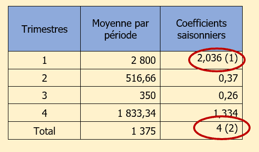
(1) : 2 800 / 1 375 = 2,036 et ainsi de suite pour chaque trimestre.
(2) : le total de la colonne coefficients saisonniers donne 4 car ce sont des chiffres d’affaires trimestriels.
La prévision des ventes se fait en prenant le chiffre d’affaires prévisionnel N+1 divisé par 4 et en le multipliant ensuite pour chaque trimestre par le coefficient du trimestre considéré.
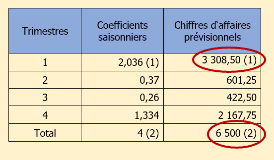
(1) : (6 500 / 4) x 2,036 = 3 308,50
(2) : selon énoncé
Le coefficient de corrélation et la prévision des ventes
Principe
Dans les 3 méthodes de prévision des ventes que nous venons de voir, le chiffre d’affaires est en relation avec le temps.
Ce n’est pas toujours le cas. Il est possible de mettre en relation le chiffre d’affaires et une autre variable.
Nous pouvons par exemple mettre en relation le chiffre d’affaires et le budget publicitaire.
Calcul du coefficient de corrélation
Le calcul du coefficient de corrélation sert à montrer si la relation, c’est à dire la dépendance, est forte entre les deux variables.
Le calcul se fait à partir d’un tableau préparatoire puis d’une formule.
Exemple de tableau préparatoire :
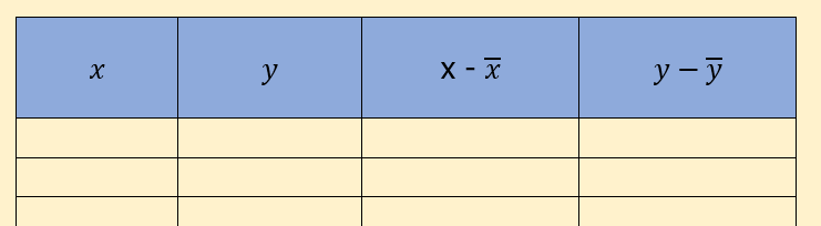
x correspond au budget publicitaire
y correspond aux chiffres d’affaires
« x barre » qui se lit « moyenne de x » correspond à la moyenne
« x – x barre » correspond à la différence entre le budget publicitaire et la moyenne des périodes
« y barre » correspond à la moyenne des chiffres d’affaires
« y – y barre » correspond à la différence entre le chiffre d’affaires et la moyenne des chiffres d’affaires
Exemple de tableau préparatoire (partie 2) :
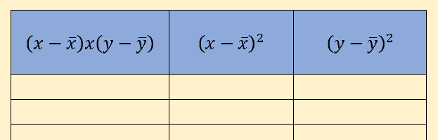
la première colonne correspond à la multiplication des variations entre la moyenne des chiffres d’affaires et la moyenne des années
la seconde colonne correspond à la différence des années et leur moyenne, le tout au carré
la dernière colonne est la différence entre le chiffre d’affaires et sa moyenne, le tout au carré
Voici la formule du coefficient de corrélation « r »:
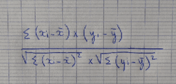
Interprétation du résultat
Le coefficient de corrélation est toujours compris entre 1 et -1.
La corrélation est forte lorsque le résultat est proche d’une des deux extrémités : 1 ou -1.
Conclusion sur la prévision des ventes
Les méthodes de prévision des ventes sont toutes les trois différentes. Chacune est utilisée dans des situations bien précises.
Si la corrélation est forte entre deux paramètres alors il est opportun de faire une prévision des ventes.
Si vous souhaitez appliquer ce que vous venez de lire, je vous invite fortement à consulter mon article sur les exercices corrigés de gestion intitulé Prévision des ventes : 6 Exercices corrigés.
Voilà, maintenant vous savez comment faire une prévision des ventes en utilisant différentes méthodes. Vous n’avez plus aucune excuse pour ne pas atteindre votre objectif : Obtenir une excellente note à l’épreuve de Gestion Opérationnelle !
Du tres bon travail. Bravo
Bonjour,
Merci à vous !
EXCELENT TRAVALLE MERCI BEAUCOUP
Bonjour KHALID OULD BOUYA,
Merci de me lire. Merci beaucoup !
Bon courage à vous.
Merci beaucoup pour la qualité de votre travail
Je vous remercie. Bon courage à vous.
Merci beaucoup pour la qualité de l’exposé!!!!
Bonjour Toure,
C’est moi qui vous remercie de me lire 🙂
Bonjour mon formateur ravie de vous retrouver sur ce nouveau exercice
La formule de a pose de problème dans d’autres exercices c’est la somme xiyi/xi2
Bonjour Nguema,
Bienvenue à nouveau,
Dans d’autres exercices du site ? Si oui de quel exercice parlez-vous svp ?
On a besoin des vidéos c’est mieux que de texte
Bonjour Yacine,
Dans ce cas là allez plutôt sur YouTube 🙂
on ne peut être plus clair, merci infiniment pour ce travail merveilleux. bon courage et bonne continuation.
Bonjour,
Je vous remercie. 🙂
Formidable article.
Merci infiniment
Bonjour Wowui,
Je vous remercie.
Bon courage.